
Disassembling EVM Bytecode (the Basics)
Recently, I’ve been looking at how to disassemble (and eventually decompile) bytecode for the Ethereum Virtual Machine (EVM). This is an interesting computer science problem which I’ve been thinking about lately. My goal is just to explain the problem and outline a simple solution.
Background
The EVM is a stack-based virtual machine which supports volatile and non-volatile storage. The volatile storage is called memory and exists only for the life of a transaction. In contrast, the non-volatile storage is just called storage and persists between transactions.
Whilst instructions in the EVM are variable length, the vast majority
are only one byte in length. The family of push instructions
(e.g. PUSH1, PUSH2, etc) are the only instructions which have
operands. These simply push a 256bit word constructed from their
operand on the stack. For example, the PUSH1 instruction accepts a
one byte operand which is converted into a 256bit word by treating the
operands as the low byte.
There are a lot of details about the EVM which I’m going to ignore
here. But, of relevance, is the fact that all branches (conditional
or unconditional) are indirect as the branch destination is
loaded from the stack. For example, if we wanted to perform an
unconditional jump to location 0x1a then we can write this:
    PUSH1 0x1a
    JUMP
In this case, the jump destination can be determined by looking at the previous instruction. But, in general, it could have been loaded onto the stack at any time in the past. For example, this is a simple variation on the above:
    PUSH1 0x1a
    PUSH1 0x80
    SLOAD
    SWAP1
    JUMP
This first loads 0x1a onto the stack, then 0x80. The SLOAD
instruction loads a word from storage at the address given on top of
the stack (0x80). To execute this instruction, the machine pops the
address and pushes the new word from storage. Say 0xff was
currently stored at 0x80, then after the SLOAD the stack is
[0x1a,0xff] (right-most element is top). The SWAP1 operation
swaps the top two stack items, so after executing this operation the
stack is [0xff,0x1a]. Finally, as before, we perform an
unconditional branch to location 0x1a.
The Problem
Performing an initial disassembly of the code is actually pretty straightforward. We can do a linear scan of the bytecode translating bytes (and operands where appropriate) into instructions. This gives us a first draft which maybe sufficient. But it lacks information which, in some cases, maybe important:
(Data vs Code). As well as executable instructions, EVM bytecode can contain data. This is often used for the contract creation process (where the code of the contract being created is stored as data), but can be used for other reasons.
(Control-Flow). Understanding the possible flow of control through the program can be important for some applications.
(Stack Height). Some applications need to know the stack height at certain points within the program.
A linear scan of bytecodes does not reveal this information. For example, it does not tell us which bytes represent actual code to execute, versus which represent data. Likewise, it does not tell us where a given branch might jump to. Furthermore, whilst a linear scan can be extended to capture some of this, we really need something more sophisticated to get reliable information.
Analysis Overview
A simple and effective solution for disassembling EVM bytecode is to use a data-flow analysis. Whilst such analyses can be quite complex, even a relatively simple dataflow analysis (such as described here) is enough for many programs.
The basic idea is to simulate execution of the bytecode using a simplified model of the machine. In fact, we’re just going to model the machine stack here and ignore memory/storage. More sophisticated analyses may want to model memory in particular (as this can reveal useful information). Our model of the machine stack is called an abstract stack (i.e. since it abstracts away information). Our abstract stack will contain concrete values (when possible) and unknown values (otherwise). Consider our program from above annotated with the state of the abstract stack before each instruction:
| Bytecode | Abstract Stack |
|---|---|
PUSH1 0x1a | [] |
PUSH1 0x80 | [0x1a] |
SLOAD | [0x1a,0x80] |
SWAP1 | [0x1a,????] |
JUMP | [????,0x1a] |
Here 0x1a and 0x80 are concrete values extracted from the PUSH1
operands, whilst ???? represents an unknown value. Since we are
simulating bytecode execution (i.e. rather than actually executing
it), we don’t know what value SLOAD will push on the stack. To
capture this safely, we abstract it with an unknown value that
represents any possible value.
The above example illustrates the main idea. Whilst our abstract
stack contains unknown values, it also contains known values. By
simulating how instructions manipulate the stack we can determine the
concrete destinations of branching instructions. For example, in the
above, the analysis tells us that the JUMP will branch to 0x1a.
Note, however, that this won’t work in all cases. For example, if the
branch address is loaded from storage, then ???? will be on top of
the stack — meaning we don’t know where the branch goes. The
essential goal is to increase analysis precision such that we can (in
many cases) determine correct branch destinations.
Control-Flow Joins
A key question arises as to what happens when different abstract stacks reach the same position in the code. Such a position is typically referred to as a join point. The following illustrates:
| Bytecode | Abstract Stack |
|---|---|
PUSH1 0x8e | [] |
PUSH1 0x1f | [0x8e] |
PUSH1 0x80 | [0x8e,0x1f] |
SLOAD | [0x8e,0x1f,0x80] |
PUSH1 0x1a | [0x8e,0x1f,????] |
JUMPI | [0x8e,0x1f,????,0x1a] |
POP | [0x8e,0x1f] |
PUSH1 0x2f | [0x8e] |
PUSH1 0x1a | [0x8e,0x2f] |
JUMP | [0x8e,0x2f,0x1a] |
This code branches to position 0x1a from two locations and, in each
case, a different abstract stack is passed along ([0x8e,0x1f] versus
[0x8e,0x2f]). It looks something like this:
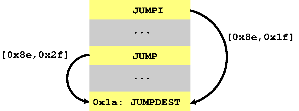
The question then is what abstract stack should we
use for location 0x1a? There are different ways we can solve this
problem, but the simplest is just to merge the two stacks together
in such a way that retains as much information as possible.
When merging two abstract stacks which have the same concrete value at
the same position, then that concrete value is retained. Otherwise,
we simply use ???? at that position (since we have no way to
represent more than one concrete value in our model). For example,
merging[0x8e,0x1f] with [0x8e,0x2f] yields the stack [0x8e,????]
which safely approximates the two possible stacks at position 0x1a.
Generalising the Abstraction
A further limitation with our abstract stack model is that it assumes a concrete stack height. Consider this variation on our program from before:
| Bytecode | Abstract Stack |
|---|---|
PUSH1 0x8e | [] |
PUSH1 0x1f | [0x8e] |
PUSH1 0x80 | [0x8e,0x1f] |
SLOAD | [0x8e,0x1f,0x80] |
PUSH1 0x1a | [0x8e,0x1f,????] |
JUMPI | [0x8e,0x1f,????,0x1a] |
SWAP1 | [0x8e,0x1f] |
POP | [0x1f,0x8e] |
PUSH1 0x1a | [0x1f] |
JUMP | [0x1f,0x1a] |
Again, this program branches to 0x1a from two locations each of
which passes along a different stack ([0x8e,0x1f] versus [0x1f]).
This looks something like this:
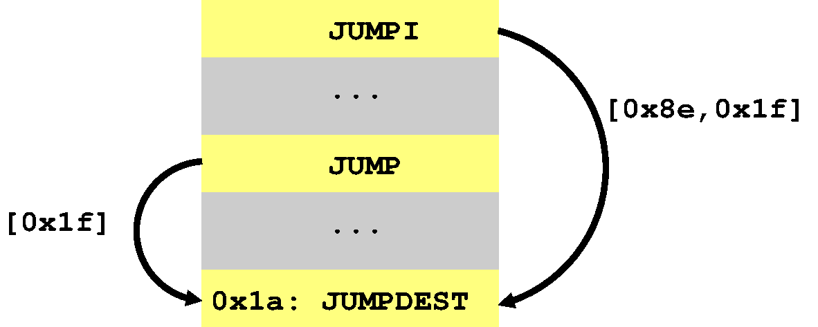
The question this time is how do we merge stacks with different
heights? With our current abstract stack model we actually can’t!
So, we need to generalise it further to support stacks of different
heights. A simple way to do this is with an integer
range l..r (where l <= r and the range
is inclusive). For example, the range 0..1 represents the set
{0,1}, whilst 0..0 represents the constant 0 (i.e. singleton set
{0}).
We can now adjust our stack model to include its length as an
integer range. For example, the stack [0x1a,0x80] in our previous
model now becomes [0x1a,0x80]:2..2 (where 2..2 signals a known
stack height of 2). This allows us to represent the merge of
[0x8e,0x1f] with [0x1f] as [0x1f]:1..2. Essentially, this
describes any stack whose top value is 0x1f and height is either 1
or 2. Anyway, there are quite a few details needed to make this
work fully, but hopefully it gives the general idea.
Conclusion
This article has given a basic overview of how dataflow analysis can be used for reasoning about jump destinations. However, to make a serious analysis which can handle bytecode found in the wild needs much more work. A good starting point for understanding this are the following papers:
- Elipmoc: advanced decompilation of Ethereum smart contracts. In Proc OOPSLA, 2022. PDF
- Gigahorse: Thorough, Declarative Decompilation of Smart Contracts. In Proc ICSE, 2019. PDF
Enjoy!
Follow the discussion on Twitter or Reddit